Read length distribution from FASTA file

Question

I have a single ~10GB FASTA file generated from an Oxford Nanopore Technologies' MinION run, with >1M reads of mean length ~8Kb. How can I quickly and efficiently calculate the distribution of read lengths?

A naive approach would be to read the FASTA file in Biopython, check the length of each sequence, store the lengths in a numpy array and plot the results using matplotlib, but this seems like reinventing the wheel.

Many solutions that work for short reads are inadequate for long reads. If I'm hey output a single (text) line per 1/10 bases, which would lead to a text output of upwards of 10,000 lines (and potentially more than 10x that) for a long read fasta.

Answer 1

If you want something quick and dirty you could rapidly index the FASTA with samtools faidx and then put the lengths column through R (other languages are available) on the command line.

samtools faidx $fasta
cut -f2 $fasta.fai | Rscript -e 'data <- as.numeric (readLines ("stdin")); summary(data); hist(data)'

This outputs a statistical summary, and creates a PDF in the current directory called Rplots.pdf, containing a histogram.

Answer 2

Statistics for nanopore reads are tricky because of the huge range of read lengths that can be present in a single run. I have found that the best way to display lengths is by using a log scale on both the x axis (length) and the y axis (sequenced bases, or counts, depending on preference).

I have written my own scripts for doing this: one for generating the read lengths, and another for plotting the length distribution in various ways. The script that generates read lengths also spits out basic length summary statistics to standard error:

$ ~/scripts/fastx-length.pl > lengths_mtDNA_called.txt
Total sequences: 2110
Total length: 5.106649 Mb
Longest sequence: 107.414 kb
Shortest sequence: 219 b
Mean Length: 2.42 kb
Median Length: 1.504 kb
N50: 336 sequences; L50: 3.644 kb
N90: 1359 sequences; L90: 1.103 kb

$ ~/scripts/length_plot.r lengths_mtDNA_called.txt
lengths_mtDNA_called.txt ... done
Number of sequences: 2110 
Length quantiles:
      0%      10%      20%      30%      40%      50%      60%      70% 
   219.0    506.9    724.4    953.0   1196.2   1503.0   1859.2   2347.3 
     80%      90%     100% 
  3128.2   4804.7 107414.0 

Here are a couple of of the produced graphs:

The scripts to generate these can be found here:

• https://github.com/gringer/bioinfscripts/blob/master/fastx-length.pl
• https://github.com/gringer/bioinfscripts/blob/master/length_plot.r

Answer 3

Using Biopython and matplotlib would seem like the way to go, indeed. It really just boils down to three lines of code to get that graph:

import Bio, pandas
lengths = map(len, Bio.SeqIO.parse('/path/to/the/seqs.fasta', 'fasta'))
pandas.Series(lengths).hist(color='gray', bins=1000)

Of course you might want to make a longer script that's callable from the command line, with a couple options. You are welcome to use mine:

#!/usr/bin/env python2

"""
A custom made script to plot the distribution of lengths
in a fasta file.

Written by Lucas Sinclair.
Kopimi.

You can use this script from the shell like this:
$ ./fastq_length_hist --input seqs.fasta --out seqs.pdf
"""

###############################################################################
# Modules #
import argparse, sys, time, getpass, locale
from argparse import RawTextHelpFormatter
from Bio import SeqIO
import pandas

# Matplotlib #
import matplotlib
matplotlib.use('Agg', warn=False)
from matplotlib import pyplot

################################################################################
desc = "fasta_length_hist v1.0"
parser = argparse.ArgumentParser(description=desc, formatter_class=RawTextHelpFormatter)

# All the required arguments #
parser.add_argument("--input", help="The fasta file to process", type=str)
parser.add_argument("--out", type=str)

# All the optional arguments #
parser.add_argument("--x_log", default=True, type=bool)
parser.add_argument("--y_log", default=True, type=bool)

# Parse it #
args        = parser.parse_args()
input_path  = args.input
output_path = args.out
x_log       = bool(args.x_log)
y_log       = bool(args.y_log)

################################################################################
# Read #
lengths = map(len, SeqIO.parse(input_path, 'fasta'))

# Report #
sys.stderr.write("Read all lengths (%i sequences)\n" % len(lengths))
sys.stderr.write("Longest sequence: %i bp\n" % max(lengths))
sys.stderr.write("Shortest sequence: %i bp\n" % min(lengths))
sys.stderr.write("Making graph...\n")

# Data #
values = pandas.Series(lengths)

# Plot #
fig   = pyplot.figure()
axes  = values.hist(color='gray', bins=1000)
fig   = pyplot.gcf()
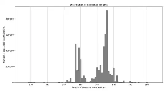
title = 'Distribution of sequence lengths'
axes.set_title(title)
axes.set_xlabel('Number of nucleotides in sequence')
axes.set_ylabel('Number of sequences with this length')
axes.xaxis.grid(False)

# Log #
if x_log: axes.set_yscale('symlog')
if y_log: axes.set_xscale('symlog')

# Adjust #
width=18.0; height=10.0; bottom=0.1; top=0.93; left=0.07; right=0.98
fig.set_figwidth(width)
fig.set_figheight(height)
fig.subplots_adjust(hspace=0.0, bottom=bottom, top=top, left=left, right=right)

# Data and source #
fig.text(0.99, 0.98, time.asctime(), horizontalalignment='right')
fig.text(0.01, 0.98, 'user: ' + getpass.getuser(), horizontalalignment='left')

# Nice digit grouping #
sep = ('x','y')
if 'x' in sep:
    locale.setlocale(locale.LC_ALL, '')
    seperate = lambda x,pos: locale.format("%d", x, grouping=True)
    axes.xaxis.set_major_formatter(matplotlib.ticker.FuncFormatter(seperate))
if 'y' in sep:
    locale.setlocale(locale.LC_ALL, '')
    seperate = lambda x,pos: locale.format("%d", x, grouping=True)
    axes.yaxis.set_major_formatter(matplotlib.ticker.FuncFormatter(seperate))

# Save it #
fig.savefig(output_path, format='pdf')

EDIT - an example output:

Answer 4

There are several potential approaches. For example:

• histogram of sequence lengths in the Biopython tutorial
• plot_distribution from the Ruby-based biopieces framework
• various solutions to get sequence length including bioawk and EMBOSS infoseq

As to which of these are "quick and efficient" using a 10 GB file...it's hard to say in advance. You may have to try and benchmark a few of them.

Answer 5

You specifically asked about FASTA files, but it's important to always consider read length and quality jointly when assessing high-error long-read data. FASTA files do not provide the quality. This information will help you determine how successful the run was, how many reads were 'high quality', etc.

I originally posted a full answer here, suggesting pauvre, but I decided it was a little off topic since you seem to only have the FASTA files.

I recommend generating FASTQ files, but I'm not sure whether you have the original base-called fast5 files. If so, generate FASTQs using poretools as follows (poretools doc for generating FASTQ files):

poretools fastq fast5/

Then I recommend generating a heat map and histogram margin plot using pauvre with both read length and quality like shown below.

[Note: I am not the original author for pauvre, but I am now contributing to this project]

Answer 6

bioawk could be reasonably efficient for this kind of task.

$ bioawk -c fastx '{histo[length($seq)]++} END {for (l in histo) print l,histo[l]}' \
    | sort -n
0   33270
1   1542
2   1132
3   3397
4   8776
5   11884
6   12474
7   14341
8   13165
9   15467
10  21089
11  30469
12  45204
13  62311
14  88744
15  115767
16  140770
17  191810
18  313088
19  518111
20  1097867
21  4729715
22  6575557
23  2734062
24  1015476
25  493323
26  323827
27  164419
28  107120
29  72487
30  40120
31  24538
32  22295
33  13121
34  9382
35  4847
36  3858
37  3161
38  2852
39  2388
40  1639
41  961
42  686
43  377
44  199
45  114
46  78
47  59
48  50
49  52
50  48
51  42
52  39
53  28
54  49
55  59
56  55
57  51
58  55
59  43
60  52
61  56
62  48
63  67
64  95
65  488

The -c fastx tells the program to parse the data as fastq or fasta. This gives access to the different parts of the records as $name, $seq (and $qual in the case of fastq format) in the awk code (bioawk is based on awk, so you can use whatever language features you want from awk).

Between the single quotes come a series of <condition> {<action>} blocks.

The first one has no <condition> part, which mean it is executed for each record. Here, it updates the lengths counts in a table which I named "histo". length is a predefined function in awk.

In the second block, the END condition means we want it to be executed after all the input has been processed. The action part consists in looping over the recorded length values and print them together with the associated count.

The output is piped to sort -n in order to sort the results numerically.

On my workstation, the above code took 20 seconds to execute for a 1.2G fasta file.

Answer 7

It is not exactly what you asked, but you can generate a histogram of read length distribution of your nanopore data directly from the HDF5 files using poretools